

Abstract
Regions of gain and loss of genomic DNA occur in many cancers and can drive the genesis and progression of disease. These copy number aberrations (CNAs) can be detected at high resolution by using microarray-based techniques. However, robust statistical approaches are needed to identify nonrandom gains and losses across multiple experiments/samples. We have developed a method called Significance Testing for Aberrant Copy number (STAC) to address this need. STAC utilizes two complementary statistics in combination with a novel search strategy. The significance of both statistics is assessed, and P-values are assigned to each location on the genome by using a multiple testing corrected permutation approach. We validate our method by using two published cancer data sets. STAC identifies genomic alterations known to be of clinical and biological significance and provides statistical support for 85% of previously reported regions. Moreover, STAC identifies numerous additional regions of significant gain/loss in these data that warrant further investigation. The P-values provided by STAC can be used to prioritize regions for follow-up study in an unbiased fashion. We conclude that STAC is a powerful tool for identifying nonrandom genomic amplifications and deletions across multiple experiments. A Java version of STAC is freely available for download at http://cbil.upenn.edu/STAC.
The accurate and unbiased identification of nonrandom subchromosomal gains and losses is important for diseases such as cancer and will likely play an increasingly important role in understanding inherited, germline copy number variation as well. Genomic copy number aberrations (CNAs) that are recurrent across individuals with a particular cancer often harbor critical disease genes whose expression level has been altered due to structural changes or abnormal gene dosage. An example is given by amplification of the MYCN oncogene in neuroblastoma that results in significant overexpression and independently predicts for high-risk and poor outcome (for review, see Maris and Matthay 1999; Brodeur and Maris 2002; Brodeur 2003). Moreover, recent evidence suggests that fixed genomic abnormalities may be more predictive of treatment response than mRNA or protein expression levels (Lynch et al. 2004; Paez et al. 2004; Winston et al. 2004). Given their role in pathogenesis, better characterization of recurrent CNAs will likely have direct clinical impact through improved patient stratification and the identification of new therapeutic targets.
Genomic copy number can be estimated for a single sample on a genome-wide scale at a high resolution using recently developed microarray-based techniques (Pinkel et al. 1998; Snijders et al. 2001; Barrett et al. 2004; Greshock et al. 2004; Ishkanian et al. 2004). Use of these methods has grown rapidly over the past few years as evidenced by the vast increase in publications found in PubMed. The computational and statistical necessities can be divided into three important steps: (1) data preprocessing, (2) single-experiment methods, and (3) multi-experiment methods. Efforts up until now have primarily focused on the first two of these. Preprocessing includes quality control and data normalization, topics that have been extensively studied in the realm of microarray analysis. Single-experiment methods are aimed at accurately identifying regions of gain and loss within an individual sample, including the optional characterization of breakpoints. There has been considerable work in this area, resulting in a wide assortment of methods, each with its own strengths and weaknesses. Approaches are often designed with an underlying platform in mind and range in complexity from simple thresholding to more sophisticated approaches that draw power from neighboring probes when making calls (for recent reviews and comparisons, see Lai et al. 2005; Willenbrock and Fridlyand 2005). These methods have been of great utility to the research community as they allow for automated copy number estimation and mapping of putative breakpoints within individual samples.
To date, however, little attention has been given to the need for multi-experiment methods to identify regions of consistent aberration across samples. Given that we are often interested in the recurrent regions of aberration, such multi-experiment methods are needed to complement the existing work on breakpoint detection in single experiments. Researchers routinely rely on simple frequency thresholds (i.e., selecting aberrations that occur in a specified percentage of the samples) for prioritizing regions for follow-up studies. This is followed by a tedious manual review of the data to define region boundaries and identify candidate genes that may be targeted by the genomic aberration. This process is time-consuming and easily prone to investigator bias. Moreover, this approach lacks the power to detect aberrant regions shared only within a subset of samples (e.g., a cancer sub-type). Multi-experiment statistical methods would provide a mechanism for accurately localizing and prioritizing recurrent aberrations in an unbiased manner thereby allowing for more focused follow-up efforts.
Here we present a new algorithm (STAC) developed to address this need. STAC identifies regions of gain or loss that occur across an entire sample set or within a subset of samples more often than would be expected under a reasonable null model. The algorithm provides a rigorous mechanism for localizing regions of significance and has been engineered to accommodate data from any array platform (e.g., BAC, SNP, oligo-based) and to handle input from any one of the previously mentioned single-experiment methods after minor data transformation. STAC includes a search of the sample space and is sensitive to concordance even if coming from only a subset of the data. We demonstrate the utility of our method by applying it to two publicly available cancer data sets for which CNAs have been published and in several cases validated experimentally. We then show how STAC can uncover additional regions of interest in these data sets, many containing known cancer-related genes. Finally, we successfully use STAC results to identify subtypes of neuroblastoma characterized by novel aberration patterns.
Results
Here we present STAC, a method for testing the statistical significance of DNA CNAs across multiple experiments. We first describe the data and notations. This is followed by a description of the null model, permutation approach, and selection of statistics. A heuristic method for searching the sample space is presented next, and we conclude with a detailed application to two publicly available cancer CNA data sets. STAC is available for download in a standalone format (STAC-Station) or a parallelized grid-based version (STAC-Grid) at http://www.cbil.upenn.edu/STAC.
Data and notations
We assume that all experimental data have been preprocessed (e.g., quality filtered and normalized) and that a method for calling gains and losses in individual samples/experiments has been applied. Therefore, our starting point is a set of aberrant regions for each sample. These data are in turn formatted for input to STAC and tested for significant concordant effects.
STAC analysis currently focuses on gain and loss as separate cases since these are generally regarded as providing distinct mechanisms for disease. We will use the term “aberration” as the generic term for both, but the type of aberration (gain or loss, considered separately) is fixed throughout this discussion. Formatted input data consist of an aberration call for each of N experiments and M fixed-width spans, which we call genomic “locations.” The sequence of M locations constitutes the stretch of genome under study and should exclude centromeres since alterations cannot be reliably detected in these regions. For cancer data we generally recommend that analysis be performed at the level of a chromosome arm, given that the observed background rate of aberration often varies considerably between arms (for examples, see aberration frequency plots in Mosse et al. 2005; Naylor et al. 2005). Analyzing each arm separately will help avoid trivial violations of our null model, such as when one arm is gained and the other is not. The width of the locations should be selected based on the resolution of the array. For example, one may select 1-Mb for a 1-Mb (on average) resolution array. In general, smaller fixed-width locations allow for finer mapping of significant regions at the cost of an increase in runtime.
We represent aberration with a 1 and no aberration with a 0. Therefore, for each stretch of genome considered and for each aberration type (gain or loss), the data can be put in an array of 0’s and 1’s where rows represent experiments and columns represent locations. We refer to a single row of this array as a “profile.” A set of consecutive 1’s in a row is called an (aberrant) “interval” for that profile. Therefore, each profile consists of a set of intervals and their locations. Figure 1 shows a graphical display of chromosome 11 loss data from a set of breast cancers consisting of N = 37 profiles and M = 77 locations. These example data are utilized below as we develop the methodology and two complementary statistics designed to test the significance of recurrent intervals of aberration.
Figure 1.

Example of chromosome 11 loss data from a set of breast cancers. Rows represent samples, and columns represent chromosomal locations. A black dot indicates there was a loss call made for that sample at that location. Consecutive black dots are connected by a line to represent an interval of aberration.
Null model and permutation approach
To calculate significance across samples, we need a statistical test that is sensitive to recurrent intervals of aberration at a given location in a selected sample set. A highly analogous problem arose in the analysis of direct identity-by-descent data, and a solution was given in Grant et al. (1999). We take the theoretical foundation laid down in that article as our starting point. As in that article, the true underlying aberration rate is not known, and we do not try to model it. Instead, we take the measured aberrations in the individual samples as given and test for the significance of consistent aberration across samples. As such, significance levels calculated are conditional on the observed data. The null model used to test for this is that the observed intervals of aberration are equally likely to occur anywhere in the stretch of the genome being considered (typically a chromosome arm). Of note, violations of this null model may include genomic regions that are inherently rearrangement-prone (Sharp et al. 2005) and those that are the sites of common deletion polymorphisms (Hinds et al. 2006; McCarroll et al. 2006). The general approach described in Grant et al. (1999) is to choose an appropriate statistic and then apply a permutation procedure under the null model to determine the significance of the statistic. For the present application, we simply need to modify the statistic and accordingly modify the search algorithm. The only heuristic involved is in the ability of the search algorithm to find the exact value of the statistic on complicated data.
An estimate of the null distribution is obtained via permutations where a permutation consists of a random rearrangement of the intervals of each profile (without replacement). In this way we preserve much of the nature of the data within samples while perturbing any concordance across samples. For example, if a profile with M locations had only one interval of length l, then there would be M − l + 1 permutations of this profile, each equally likely.
The frequency statistic
The first statistic we consider associates to each location m the frequency of aberration at that location across the entire sample set, denoted F(m). Extreme values of the statistic F(m) indicate deviation from the null model at location m.If P is a permutation of the data, we denote the frequency of aberration in the permuted data over location m by FP(m), m = 1 … M. Let D be the distribution (over all permutations P) of maxm FP(m). In other words, D is the permutation distribution of the maximum aberration frequency. We define a frequency-based P-value at each location m0, denoted P F(m 0), by the right-hand tail probability of F(m0) in D
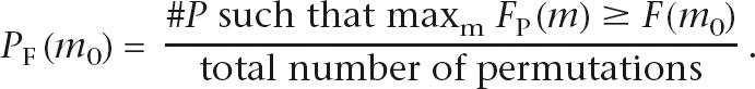 |
Since we are comparing F(m 0) to the distribution of the maximum aberration frequency over all m, the resulting P-value P F(m 0) is a multiple testing corrected confidence measure (for the M tests) for rejection of the null model. Since our statistic is an indicator of behavior at location m0, we prioritize the locations by the P F(m 0). If location m0 is significant to level α (e.g., 0.05 or 0.01), then location m0 has a frequency that is unlikely under the null model indicating possible biological significance.
We define the “confidence” at location m0 as 1 − P F(m 0). Figure 2A shows the data from Figure 1 with the frequency confidences overlaid as gray bars. Four intervals of significant loss are identified and suggest putative locations for cancer-related genes. One can also see from these data that the frequency is not significant at the three leftmost locations (marked by *); however, there is a consistent aberration within a subset of nine samples. Given that cancers are often heterogeneous and copy number profiles can be used to discover and distinguish subtypes, it is imperative that one be able to identify this type of alteration in addition to those that are significantly frequent across the entire sample set.
Figure 2.

Results for example data using frequency and footprint statistics. Display showing data from Figure 1 with overlay of the confidences, indicated by gray bars. The red line graphs the actual frequencies in the sample set. (A) Frequency only. (B) Footprint only.
The footprint and the normalized footprint
To overcome the shortcoming of the global frequency statistic outlined at the end of the previous section, we develop a refined version of the “footprint” statistic and subset search methodology originally introduced by Grant et al. (1999). Although the biological question here is different, the data and statistical problems that arise from them are similar.
We define a “stack,” S, as a set of intervals that contains at most one interval per profile and where there is at least one location common to every interval in the set. Note that in Grant et al. (1999) the second requirement is not imposed. A stack is not necessarily composed of all intervals over a location, it can contain any subset of them. We define the footprint of a stack S, denoted by F(S), to be the number of locations c such that c is contained in some interval of S (see Fig. 3A). The footprint accounts for interval lengths and measures tight alignment as a much more significant case than the aberration frequency. Figure 3B illustrates this advantage. The aberration frequency at the position in red is four in both examples. However, the footprint of the stack on the right is much smaller than the footprint of the stack on the left, emphasizing the unlikely scenario of this tight alignment if aberrations occurred randomly. The notion of tight alignment is useful for localizing regions of significance and narrowing the list of candidate genes that may be targeted by the genomic aberration. Although the location in red may harbor a critical gene based on the data on the left, the data on the right provide greater evidence for this localization and this is reflected in its smaller footprint.
Figure 3.

Footprint of a stack. (A) The footprint of a stack is the number of locations contained in some interval of the stack. The anchor point(s) of a stack are the locations contained in every interval of the stack. Black dotted line represents a stretch of genome. Gray dotted lines represent aberrant intervals. (B) Footprint accounts for interval lengths. Two example stacks are shown; “frequency” and “footprint” indicate values of frequency and footprint, respectively. Both stacks cover the location indicated in red; however, the stack on the right provides greater evidence for localization of an important gene at this location; this is reflected in its smaller footprint.
The requirement that stacks be anchored mitigates the need for normalization of the footprint as introduced in Grant et al. (1999); however, it is still necessary in order to put similar stacks on equal footing regardless of interval length. Consider, for example, two stacks containing the same number of intervals, the first a perfectly aligned stack of intervals of length one and the second a perfectly aligned stack of intervals of length two. The first stack has a footprint that is half that of the second; however, both stacks provide strong evidence of a nonrandom effect and the potential localization of an important gene. To avoid overemphasizing the difference in widths, we normalize the footprint by dividing by its expected value NF(S) = F(S)/E(F(S)), where the expected value is calculated under the usual null model. In this way, the normalized footprint of the first stack in our example is only slightly smaller than the normalized footprint of the second stack.
Footprint-based P-values
Ultimately we would like to assess the significance of recurrent intervals of aberration at each location. However, the normalized footprint, when applied only to the set of all intervals covering a given location, is not sensitive enough for this purpose. Suppose there is one profile that has a very long interval (a scenario common in cancer data sets). Then this interval will cause the footprint (as well as the normalized footprint) to be large regardless of the other intervals involved. We therefore do not apply the normalized footprint to all intervals over each location, but rather we apply it to each stack, regardless of how many profiles/ intervals are involved. We then test the value of the normalized footprint on each stack for significance with respect to the usual null model; these data in turn are used to assess significance at each location.
For any stack S, we call m an anchor point of the stack if m is contained in every interval. We denote the set of all anchor points of a stack S by S*. By the definition of a stack given in the previous section, S* ≠ Ø. Let Dn, n = 2 … N be the permutation distribution of NF(S) over all stacks S that consist of exactly n intervals. For each stack S in the unpermuted data containing n intervals, let P(S)bethe P-value given by the tail probability in Dn for values ≤ NF(S). P(S) is a permutation P-value assigned to a stack; these P-values can be used to assess significance at each location in S* as follows. For each location m, let
R provides a uniform P-value–based score that makes all locations comparable, regardless of the nature of the stacks over them. We cannot use the score as a meaningful P-value, however, since they are not multiple testing corrected for taking a minimum over all subset sizes. Therefore we perform a second permutation calculation on the R(m) themselves in order to assess true significance. Since R is a score for each location, much as the frequency is, we assess the significance of R in exactly the same way as we did with the frequency. This provides us with a footprint-based P-value at each location. It is important to note that a location may derive significance from either a subset of samples or the entire sample set given that we are evaluating stacks of all possible sizes (i.e., containing any number of samples).
Searching the sample space
A search method averts the only serious obstacle in calculating the footprint-based P-values, which is the impossibility (except in simple cases) of searching, for each n, the astronomically large space of all stacks S that consist of exactly n intervals. This problem only arises with the footprint statistic since the frequency does not require a subset search. We use a similar search strategy as in Grant et al. (1999) with an additional step to remove redundancy at each level. Two stacks S 1 and S 2 are considered redundant if they comprised the same number of intervals and share the same anchor points, and the set of interval lengths for intervals contained in S 1 equals that of S 2.
The approach is heuristic and searches the sample space in a greedy and incremental manner from 2 to N (i.e., the maximum possible stack size). For B, a fixed positive integer, it starts by finding the best B anchored stacks involving two intervals; “best” meaning with smallest normalized footprint. The algorithm then extends those B stacks in all possible ways to anchored stacks involving three intervals and finds the best nonredundant B of those. Those B stacks of three intervals are in turn extended to all anchored stacks of four intervals, and the best B nonredundant of those are determined. This process continues incrementally up to the largest possible stack. The minimum normalized footprint found at each step is recorded. These are the NF(S) values used above in the distributions D n.
The removal of redundancy is a necessary step, particularly for large data sets. Because the number of substacks of a stack grows exponentially with the size of the stack, if redundancy is not removed, then the best B stacks considered for extension at a level could consist entirely of stacks anchored at the same location(s). Extending only these stacks to the next level could result in false negatives elsewhere on the chromosome arm. Note that the removal of redundancy does not bias our P-values because the same search strategy is applied to both the permuted and unpermuted data.
Optimization of this process can be achieved through the review and testing of the “search parameter” B. The higher B is set the more likely it is to find the global minimum, but the longer it will take to run. The appropriate setting of B will depend on the particular data set being analyzed, and STAC provides output that can help guide this decision. For example, one can output the number of stacks considered for extension at each level. From this, one can determine at which level of extension the heuristic will begin to take affect. In practice, we have found that setting B = 10,000 is more than sufficient for most data sets consisting of ∼50 samples.
Figure 2B shows the results for the example data using footprint-based confidences alone. Notice how the locations at the left that were not significantly frequent across the entire data set are now found to be significant using the normalized footprint and subset search. In addition, another stack has been revealed (marked by *) that was less apparent and that we might have missed by eye. These locations may be relevant to a distinct subgroup of the samples.
In practice, we find the frequency and footprint statistics complement one another. We therefore report the results for both statistics. Deriving meaningful and effective conclusions requires the careful consideration of both statistics since the inherent statistical meaning (and therefore biological implication) of each is different.
Application to two publicly available cancer CNA data sets
We applied our algorithm to two publicly available cancer CNA data sets. The first consists of CNA data from 42 cell lines derived from diagnostic or relapsed neuroblastomas (Mosse et al. 2005). The second set is generated from 47 primary sporadic breast tumors (Naylor et al. 2005). Original CNA data were preprocessed to generate appropriate input data for STAC as described in the Methods section. For each chromosome arm, STAC was executed separately for gains and losses. We set the search parameter to 10,000 and performed 10,000 random permutations to assess the significance of both statistics (for timing results, see Supplemental Table 1). A location with P-value ≤ 0.05 for either statistic was considered significant, and we use P fr and P fp to designate the frequency and footprint-based P-values, respectively.
Table 1.
Comparison to previously reported regions in neuroblastoma data set

STAC detects regions of known biological and clinical relevance
We first sought to investigate whether STAC could identify known clinically and biologically relevant genomic aberrations. Specifically, we expect to identify amplification at 2p24 containing MYCN, loss at 1p36, loss at 11q14–25, and gain of 17q material in the neuroblastoma data, as these aberrations have been shown to be clinically and/or biologically relevant (for review, see Maris and Matthay 1999).
Figure 4 shows the results for the four chromosome arms studied. STAC successfully finds locations of significance for each relevant chromosomal region. Amplification at 2p24 including the MYCN oncogene is readily identified (P fp = 0.0003, P fr = 0.0001), as is the region of loss at 1p36 (P fp = 0.0014, P fr = 0.0028), Analysis of chromosome arms 11q and 17q reveals the complementary nature of the statistics employed by STAC. Given the frequency of 17q gain, it seems clear that this aberration plays an important role in neuroblastoma. However, the problem of localizing a region (or regions) that may harbor putative oncogenes is far more difficult given the large intervals of gain seen in most samples. STAC identifies three relatively small regions of significant gain at 17q24.1 (P fp = 0.0102), 17q24.2 (P fp = 0.0075), and 17q25 (P fp = 0.0348) based on the footprint. Similarly, while a small region of loss is detected by both statistics at 11q23.3 (P fp = 0.0193, P fr = 0.0181), identification of the regions at 11q14.3–11q21 (P fp = 0.0005) and 11q25 (P fp = 0.0023) requires the increased sensitivity of the footprint statistic. All regions identified by STAC are within currently accepted significant regions of overlap (SROs) in neuroblastoma. Moreover, these data potentially narrow the regions and provide a mechanism for prioritizing follow-up efforts.
Figure 4.

STAC identifies clinically and biologically relevant regions in neuroblastoma. For each arm studied, 1-Mb locations are plotted along the x-axis, and each sample having at least one interval of aberration along the chromosome arm is plotted on the y-axis. The gray bars track the maximum STAC confidence (1 − P-value), darker bars are those with confidence >0.95. Locations indicated at the top by a red bar designate significant stacks falling within (or spanning) regions of known biological and/or clinical relevance. Locations indicated at the bottom by a blue bar were found significant only by the footprint. (A) 1p loss; (B) 2p gain; (C) 11q loss; (D) 17q gain.
STAC provides statistical support for previously reported CNAs
As a further validation step, we compare regions identified previously by Mosse et al. (2005) and Naylor et al. (2005) using traditional frequency thresholding and manual review to our STAC results for these data sets. For each previously reported region, we examine the STAC results to see if statistical support is present. In all cases, we consider a P-value ≤ 0.05 for either statistic as significant.
STAC provides statistical support for the majority of the regions reported in Mosse et al. (2005), who defined regions of gain/loss in the neuroblastoma data based on a frequency cutoff of 25%. In other words, the aberration must be observed in 25% of the cell lines considered. Region boundaries were then determined based on manual inspection. Our analysis provides statistical support for 86.9% (20 of 23) of the gain regions and 91.7% (11 of 12) of the loss regions (Table 1).
STAC results for each of the 25 regions reported by Naylor et al. (2005) for the breast cancer data show a high degree of concordance (Table 2). Published regions were based on a frequency cutoff of 30% and tedious manual review to define region boundaries. STAC provides statistical support for 91.7% (11 of 12) of the gains regions and 76.9% (10 of 13) of the loss regions previously reported. In addition, Naylor et al. reported a full set of 55 regions of gain as supplemental data, for which STAC finds statistical support for 82% (45 of 55); for details, see Supplemental Table 2.
Table 2.
Comparison to previously reported regions in breast cancer data set

Examination of the few discordant regions revealed two reasons for discrepancy. The most common explanation is the presence of frequent and long aberrant intervals, such as seen in the neuroblastoma data for 17q gains. Here, 90% of the cell lines exhibit large gains, rendering the localization of regions near impossible without statistical methods. The discordant region (54.5–57.7 Mb) was gained in ∼70% of the samples, yet our STAC frequency statistic tells us that this occurs 95% of the time in randomly permuted data. Manual review of such data to define regions is easily subject to investigator bias. The second explanation for discrepancy is simply that the region fell just below our P-value cutoff for significance. For example, loss on 3p reported in Mosse et al. (2005) is assigned P fr = 0.0698 by STAC. It is possible that this region would reach significance with the power gained by additional samples.
STAC identifies additional regions of significant gain/loss
We hypothesize that traditional methods could miss many regions of statistical significance and likely biological relevance. We therefore characterize all regions of significant gain and loss identified in our analysis (for a global view, see Supplemental Fig. 1).
STAC finds a total of 94 regions of significant gain and 79 regions of significant loss in the neuroblastoma data (Supplemental Table 3). The gains encompass a total of 332 Mb of genomic sequence with an average region size of 3.53 Mb. Significant loss covers 305 Mb of genomic sequence with an average region size of 3.86 Mb. Of note, 77% (72 of 94) of the gain regions and 86% (69 of 80) of the loss regions went undetected by the traditional frequency threshold approach.
Supplemental Table 4 provides a complete listing of all regions identified in the sporadic primary breast tumor data set. In summary, STAC analysis identifies 149 distinct regions of significant gain covering 525 Mb of genomic sequence. The average region of gain spans 3.43 Mb, and 94 of the regions found by STAC were not identified by a simple frequency thresholding approach. Our analysis identifies 124 distinct regions of loss covering 383 Mb of genomic sequence. The average region of loss spans 3.10 Mb.
Biological relevance of additional regions found by STAC
We sought to determine if the additional regions found by STAC have biological meaning. Ideally, this is done by using a large panel of highly annotated samples where one can then test whether regions are correlated with clinically and biologically relevant subsets and/or patient outcome. Here, we utilize what is known about neuroblastoma both cytogenetically and clinically to guide our biological interpretation of significant STAC regions.
We performed two-way agglomerative hierarchical clustering on the significant STAC regions to facilitate the biological interpretation of our neuroblastoma STAC results (Fig. 5). Two clusters of samples characterized by distinct patterns of gain and loss are observed (Fig. 5A). Regions of known biological and clinical relevance are shown in Figure 5B, A through D. Sample clustering is not driven by gain of the MYCN oncogene at 2p24 (A) or 17q gain (B), both very frequent events in this data set. Samples with 1p36 loss (D) are clearly separated from those with 11q loss (C); it is well established that these genomic aberrations are negatively correlated and associated with poor prognosis in neuroblastoma (for review, see Maris and Matthay 1999). Thus, we have confidence that the sample clusters are explained in part by known biology.
Figure 5.

Unsupervised two-way hierarchical clustering of 42 neuroblastoma (NB) cell lines based on significant STAC regions of gain and loss. (A) Two main sample clusters. (B) Known clinically and/or biologically relevant regions. (C) Additional regions characterizing two sample clusters. Labels A–E represent locations present in zoomed image. A and B represent known gains in NB. C and D represent known losses in NB that are negatively correlated. E′ indicates that only a subset of locations from E are displayed. **Significant by STAC analysis, but not reported in Mosse et al. (2005).
Sample cluster 1 is characterized by regions of loss, whereas cluster 2 exhibits frequent gain at these same locations (Fig. 5A, location cluster labeled E). Two thirds (145/217) of the locations contained in E were not identified by Mosse et al. (2005) using a frequency threshold of 25%. The fact that these regions associate with aberrations of known biological and clinical relevance in this data set indicates they may warrant further investigation. Figure 5C provides a zoomed display of eight randomly selected regions from “E”. Five of the eight regions (marked by **) are detected by STAC but missed by traditional frequency thresholding. These data suggest that gains on chr20, 15, 16, 13, and 22 may be negatively associated with loss at 1p36 and could represent two distinct progression pathways in neuroblastoma.
Discussion
Cancer genomes are often riddled with CNAs, rendering the identification of relevant regions across multiple samples extremely difficult. Researchers traditionally rely on a simple frequency cutoff (e.g., “deleted in 30% of samples”) followed by a laborious manual review to define region boundaries. While this approach may identify some relevant locations, it is tedious and time-consuming and lacks statistical control over false positives and false negatives. In particular, it assumes a constant null model across the genome, and therefore is too liberal in some cases and too conservative in others.
We propose a sensitive statistical method for assessing the significance of recurrent genomic CNAs. STAC readily identifies regions of known biological and clinical relevance and reveals new recurrent aberrations that warrant further investigation. The method is sensitive to tight alignment of aberrant intervals and is capable of finding consistent regions of aberration within subsets of samples/experiments. These features are essential for localizing cancer genes and understanding cancer subtypes and progression. As with any computational analysis of large-scale data, STAC results should be reviewed to assess potential biological relevance. Not all significantly concordant aberrations may be relevant to the problem at hand. For example, STAC may identify copy number polymorphisms (CNPs) in addition to the recurrent CNAs that are the focus of cancer studies. Also, it is possible that some of the regions found by STAC represent artifacts of array fabrication/hybridization, the binning into fixed-width locations, or inaccuracies in the input data that our significance calculations are based on. However, unsupervised clustering of STAC results from neuroblastoma cell lines suggests that many of the additional regions have biological significance. Evidence for this is provided by their correlation with genomic abnormalities known to be associated with high-risk and poor outcome. Additional studies in a large panel of tumor specimens are underway to confirm this.
Few others have attempted to address the multi-experiment problem computationally (Aguirre et al. 2004; Lipson et al. 2005; Rouveirol et al. 2006). Aguirre et al. (2004) propose a rule-based method for identifying minimal common regions (MCRs) and suggest criteria for prioritizing MCRs. They assess the significance of the median log2-ratios across experiments for each MCR; however their overall approach is largely heuristic. Lipson et al. (2005) define a statistical framework involving the use of interval scores to address both the single and multi-experiment problems. This solution relies on untested parametric assumptions and does not make multiple testing considerations; therefore it is impossible to assess the true error rate of the method. Rouveirol et al. (2006) recently formalized two algorithms for identifying MCRs; however they do not involve any statistical significance testing. Neither method of Aguirre et al. or Lipson et al. has been implemented in a publicly available form to date.
It is important to note that all multi-experiment approaches currently require one to first define the gains and losses within each individual sample. The best approach for doing this has yet to be determined and depends on the particular array and experimental design. We have found that the use of ratio thresholds for calling gain and loss often leads to false negatives (missing regions of aberration in individual samples) and can also lead to false positives, depending on experimental design. Concordant bias such as that which may be introduced by severe sample processing should be accounted for. For example, if the probe distributions are significantly variable, one can hybridize a battery of normal controls (processed identically to the test samples) in order to use a standard deviation criterion instead of a global ratio cutoff. It is often preferable to use one of the model-based methods to make gain/loss calls for each sample; however, this can result in a decrease in resolution since they tend to not call a region as aberrant unless it is supported by several array elements. In general, given that concordant bias has been minimized as described above, the single slide calls should be made fairly liberally, so to avoid false negatives, since the false positives in individual samples will be randomly scattered across the genome and STAC will not assign significance to these additional aberrations. In short, if it is just noise in the array, it does not result in STAC false positives.
We envision at least two extensions to STAC in the near future. We first plan to enhance the power of STAC by incorporating the degree of gain and loss at each interval, especially high-level amplification and homozygous deletion. This can be accomplished by modifying our statistics to account for weighted intervals, where the weight of an interval is reflective of its degree of gain/loss. This is an intuitive extension to our method given that researchers routinely give greater consideration to more extreme alterations. The second planned extension is the assessment of significant co-occurring aberrations across multiple experiments. Such shared aberrations can be indicative of distinct disease progression pathways and as such are of obvious interest.
Lastly, we note that our algorithm is applicable to genomic research beyond cancer and the study of other diseases. Recent studies utilizing genomic copy number data from normal populations have noted the extent of genomic CNPs in the human genome and that CNPs are enriched near regions of segmental duplication (Bailey et al. 2002; Sharp et al. 2005). STAC analysis of copy number data from normal individuals would provide statistical rigor to these studies and may reveal new CNPs and potential patterns of CNPs within populations and/or population subsets. Moreover, STAC addresses the need to search for concordant effects in a fairly generic manner. Given that this type of problem arises in the analysis of other genomic-related data (e.g., methylation and IBD), STAC may also be useful beyond the realm of genomic copy number analysis.
Methods
Validation genomic CNA data
Array-CGH data from 42 neuroblastoma cell lines (Mosse et al. 2005) and 47 sporadic primary breast tumors (Naylor et al. 2005) were used to validate and illustrate our method. The details of array design, fabrication and hybridization protocols have been described in detail previously (Greshock et al. 2004). The method for calling gains and losses for each individual sample has also been described previously (Mosse et al. 2005; Naylor et al. 2005). These data are used for validation purposes and can be downloaded from http://acgh.afcri.upenn.edu/nbacgh (neuroblastoma) and http://acgh.afcri.upenn.edu/bracgh (breast).
Data preprocessing
Given the resolution of the arrays used for the validation data (1-Mb), we selected 1-Mb as the size of each fixed-width location. Heterochromatic centromere regions were excluded from analysis given the lack of probes present on the array. Cytoband information (“cytoband.txt”) was downloaded from http://genome.ucsc.edu for build 16 of the human genome (July 2003 freeze). Regions designated “acen” were excluded from our analysis. As per the original publications, chromosomes X and Y were excluded from analysis, along with the short arms of acrocentric chromosomes 13, 14, 15, 21, and 22. To be consistent with the original publications, all genomic coordinates used in our analysis are based on UCSC Genome Browser build 16 (July 2003 freeze) of the human genome.
Unsupervised class discovery
Unsupervised two-way agglomerative hierarchical clustering using complete linkage with Pearson's correlation as a similarity metric was performed by using Cluster (Eisen et al. 1998). We first filtered the 1-Mb locations across the genome to include only those found significantly aberrant by STAC and having a minimum stack size of 4. This resulted in a reduction from 2.7 Gb to 588 Mb. Input data for clustering then consisted of trinary calls of (−1, 0, 1) for loss, no change, and gain for each significant location. In the rare case that a sample exhibited both gain and loss within the location (<0.1%), we did not make a call but instead indicated these as missing values due to their ambiguity. The resulting clustering was visualized by using TreeView.
Acknowledgments
We thank Mitchell Guttman for important bug reports and Warren J. Ewens for his guidance and useful discussions. This work was supported in part by NIH/NHGRI Training Grant in Computational Genomics 2-T32-HG000046-07 (S.J.D.), K25-HG-0052 (G.R.G., the Abramson Family Cancer Research Institute (B.L.W., J.M.M.), and a seed grant provided by the Penn Genomics Institute (PGI) of the University of Pennsylvania.
Footnotes
[Supplemental material is available online at www.genome.org.]
Article published online before print. Article and publication date are at http://www.genome.org/cgi/doi/10.1101/gr.5076506. Freely available online through the Genome Research Open Access option.
References
- Aguirre A.J., Brennan C., Baily G., Sinha R., Feng B., Leo C., Zhang Y., Zhang J., Gans J.D., Bardessy N., Brennan C., Baily G., Sinha R., Feng B., Leo C., Zhang Y., Zhang J., Gans J.D., Bardessy N., Baily G., Sinha R., Feng B., Leo C., Zhang Y., Zhang J., Gans J.D., Bardessy N., Sinha R., Feng B., Leo C., Zhang Y., Zhang J., Gans J.D., Bardessy N., Feng B., Leo C., Zhang Y., Zhang J., Gans J.D., Bardessy N., Leo C., Zhang Y., Zhang J., Gans J.D., Bardessy N., Zhang Y., Zhang J., Gans J.D., Bardessy N., Zhang J., Gans J.D., Bardessy N., Gans J.D., Bardessy N., Bardessy N., et al. High-resolution characterization of the pancreatic adenocarcinoma genome. Proc. Natl. Acad. Sci. 2004;101:9067–9072. doi: 10.1073/pnas.0402932101. [DOI] [PMC free article] [PubMed] [Google Scholar]
- Bailey J.A., Gu Z., Clark R.A., Reinert K., Samonte R.V., Schwartz S., Adams M.D., Meyers E.W., Li P.W., Eichler E.E., Gu Z., Clark R.A., Reinert K., Samonte R.V., Schwartz S., Adams M.D., Meyers E.W., Li P.W., Eichler E.E., Clark R.A., Reinert K., Samonte R.V., Schwartz S., Adams M.D., Meyers E.W., Li P.W., Eichler E.E., Reinert K., Samonte R.V., Schwartz S., Adams M.D., Meyers E.W., Li P.W., Eichler E.E., Samonte R.V., Schwartz S., Adams M.D., Meyers E.W., Li P.W., Eichler E.E., Schwartz S., Adams M.D., Meyers E.W., Li P.W., Eichler E.E., Adams M.D., Meyers E.W., Li P.W., Eichler E.E., Meyers E.W., Li P.W., Eichler E.E., Li P.W., Eichler E.E., Eichler E.E. Recent segmental duplications in the human genome. Science. 2002;297:1003–1007. doi: 10.1126/science.1072047. [DOI] [PubMed] [Google Scholar]
- Barrett M.T., Scheffer A., Ben-Dor A., Sampas N., Lipson D., Kincaid R., Tsang P., Curry B., Baird K., Meltzer P.S., Scheffer A., Ben-Dor A., Sampas N., Lipson D., Kincaid R., Tsang P., Curry B., Baird K., Meltzer P.S., Ben-Dor A., Sampas N., Lipson D., Kincaid R., Tsang P., Curry B., Baird K., Meltzer P.S., Sampas N., Lipson D., Kincaid R., Tsang P., Curry B., Baird K., Meltzer P.S., Lipson D., Kincaid R., Tsang P., Curry B., Baird K., Meltzer P.S., Kincaid R., Tsang P., Curry B., Baird K., Meltzer P.S., Tsang P., Curry B., Baird K., Meltzer P.S., Curry B., Baird K., Meltzer P.S., Baird K., Meltzer P.S., Meltzer P.S., et al. Comparative genomic hybridization using oligonucleotide microarrays and total genomic DNA. Proc. Natl. Acad. Sci. 2004;101:17765–17770. doi: 10.1073/pnas.0407979101. [DOI] [PMC free article] [PubMed] [Google Scholar]
- Brodeur G.M. Neuroblastoma: Biological insights into a clinical enigma. Nat. Rev. Cancer. 2003;3:203–216. doi: 10.1038/nrc1014. [DOI] [PubMed] [Google Scholar]
- Brodeur G.M., Maris J.M., Maris J.M. In: Principles and practice of pediatric oncology. 4th ed. Pizzo P.A., Pollack D.G., Pollack D.G., editors. Lippincott Williams & Wilkins; Philadelphia PA: 2002. pp. 895–938. [Google Scholar]
- Eisen M.B., Spellman P.T., Brown P.O., Botstein D., Spellman P.T., Brown P.O., Botstein D., Brown P.O., Botstein D., Botstein D. Cluster analysis and display of genome-wide expression patterns. Proc. Natl. Acad. Sci. 1998;95:14863–14868. doi: 10.1073/pnas.95.25.14863. [DOI] [PMC free article] [PubMed] [Google Scholar]
- Grant G., Manduchi E., Cheung V., Ewens W., Manduchi E., Cheung V., Ewens W., Cheung V., Ewens W., Ewens W. Significance testing for direct identity-by-descent mapping. Ann. Hum. Genet. 1999;63:441–454. doi: 10.1046/j.1469-1809.1999.6350441.x. [DOI] [PubMed] [Google Scholar]
- Greshock J., Naylor T., Margolin A., Diskin S., Cleaver S.H., Futreal P.A., deJong P.J., Zhao S., Liebman M., Weber B.L., Naylor T., Margolin A., Diskin S., Cleaver S.H., Futreal P.A., deJong P.J., Zhao S., Liebman M., Weber B.L., Margolin A., Diskin S., Cleaver S.H., Futreal P.A., deJong P.J., Zhao S., Liebman M., Weber B.L., Diskin S., Cleaver S.H., Futreal P.A., deJong P.J., Zhao S., Liebman M., Weber B.L., Cleaver S.H., Futreal P.A., deJong P.J., Zhao S., Liebman M., Weber B.L., Futreal P.A., deJong P.J., Zhao S., Liebman M., Weber B.L., deJong P.J., Zhao S., Liebman M., Weber B.L., Zhao S., Liebman M., Weber B.L., Liebman M., Weber B.L., Weber B.L. 1-Mb resolution array-based comparative genomic hybridization using a BAC clone set optimized for cancer gene analysis. Genome Res. 2004;14:179–187. doi: 10.1101/gr.1847304. [DOI] [PMC free article] [PubMed] [Google Scholar]
- Hinds D.A., Kloek A.P., Jen M., Chen X., Frazer K.A., Kloek A.P., Jen M., Chen X., Frazer K.A., Jen M., Chen X., Frazer K.A., Chen X., Frazer K.A., Frazer K.A. Common deletions and SNPs are in linkage disequilibrium in the human genome. Nat. Genet. 2006;38:82–85. doi: 10.1038/ng1695. [DOI] [PubMed] [Google Scholar]
- Ishkanian A.S., Malloff C.A., Watson S.K., DeLeeuw R.J., Chi B., Coe B.P., Snijders A., Albertson D.G., Pinkel D., Marra M.A., Malloff C.A., Watson S.K., DeLeeuw R.J., Chi B., Coe B.P., Snijders A., Albertson D.G., Pinkel D., Marra M.A., Watson S.K., DeLeeuw R.J., Chi B., Coe B.P., Snijders A., Albertson D.G., Pinkel D., Marra M.A., DeLeeuw R.J., Chi B., Coe B.P., Snijders A., Albertson D.G., Pinkel D., Marra M.A., Chi B., Coe B.P., Snijders A., Albertson D.G., Pinkel D., Marra M.A., Coe B.P., Snijders A., Albertson D.G., Pinkel D., Marra M.A., Snijders A., Albertson D.G., Pinkel D., Marra M.A., Albertson D.G., Pinkel D., Marra M.A., Pinkel D., Marra M.A., Marra M.A., et al. A tiling resolution DNA microarray with complete coverage of the human genome. Nat. Genet. 2004;36:299–303. doi: 10.1038/ng1307. [DOI] [PubMed] [Google Scholar]
- Lai W.R., Johnson M.D., Kucherlapati R., Park P.J., Johnson M.D., Kucherlapati R., Park P.J., Kucherlapati R., Park P.J., Park P.J. Comparative analysis of algorithms for identifying amplifications and deletions in array CGH data. Bioinformatics. 2005;19:3763–3770. doi: 10.1093/bioinformatics/bti611. [DOI] [PMC free article] [PubMed] [Google Scholar]
- Lipson D., Aumann Y., Ben-Dor A., Linial N., Yakhini Z., Aumann Y., Ben-Dor A., Linial N., Yakhini Z., Ben-Dor A., Linial N., Yakhini Z., Linial N., Yakhini Z., Yakhini Z. Proceedings of RECOMB ‘05. Springer-Verlag; Cambridge MA: 2005. Efficient calculation of interval scores for DNA copy number data analysis. [Google Scholar]
- Lynch T.J., Bell D.W., Sordella R., Gurubhagavatula S., Okimoto R.A., Brannigan B.W., Haris P.L., Haserlat S.M., Supko J.G., Haluska F.G., Bell D.W., Sordella R., Gurubhagavatula S., Okimoto R.A., Brannigan B.W., Haris P.L., Haserlat S.M., Supko J.G., Haluska F.G., Sordella R., Gurubhagavatula S., Okimoto R.A., Brannigan B.W., Haris P.L., Haserlat S.M., Supko J.G., Haluska F.G., Gurubhagavatula S., Okimoto R.A., Brannigan B.W., Haris P.L., Haserlat S.M., Supko J.G., Haluska F.G., Okimoto R.A., Brannigan B.W., Haris P.L., Haserlat S.M., Supko J.G., Haluska F.G., Brannigan B.W., Haris P.L., Haserlat S.M., Supko J.G., Haluska F.G., Haris P.L., Haserlat S.M., Supko J.G., Haluska F.G., Haserlat S.M., Supko J.G., Haluska F.G., Supko J.G., Haluska F.G., Haluska F.G., et al. Activating mutations in the epidermal growth factor receptor underlying responsiveness of non-small-cell lung cancer to gefitinib. N. Engl. J. Med. 2004;350:2129–2139. doi: 10.1056/NEJMoa040938. [DOI] [PubMed] [Google Scholar]
- Maris J.M., Matthay K.K., Matthay K.K. Molecular biology of neuroblastoma. J. Clin. Oncol. 1999;17:2264–2279. doi: 10.1200/JCO.1999.17.7.2264. [DOI] [PubMed] [Google Scholar]
- McCarroll S.A., Hadnott T.N., Perry G.H., Sabeti P.C., Zody M.C., Barrett J.C., Dallaire S., Gabriel S.B., Lee C., Daly M.J., Hadnott T.N., Perry G.H., Sabeti P.C., Zody M.C., Barrett J.C., Dallaire S., Gabriel S.B., Lee C., Daly M.J., Perry G.H., Sabeti P.C., Zody M.C., Barrett J.C., Dallaire S., Gabriel S.B., Lee C., Daly M.J., Sabeti P.C., Zody M.C., Barrett J.C., Dallaire S., Gabriel S.B., Lee C., Daly M.J., Zody M.C., Barrett J.C., Dallaire S., Gabriel S.B., Lee C., Daly M.J., Barrett J.C., Dallaire S., Gabriel S.B., Lee C., Daly M.J., Dallaire S., Gabriel S.B., Lee C., Daly M.J., Gabriel S.B., Lee C., Daly M.J., Lee C., Daly M.J., Daly M.J., et al. Common deletion polymorphisms in the human genome. Nat. Genet. 2006;38:86–92. doi: 10.1038/ng1696. [DOI] [PubMed] [Google Scholar]
- Mosse Y.P., Greshock J., Margolin A., Naylor T., Cole K., Khazi D., Hii G., Winter C., Shahzad S., Asziz M.U., Greshock J., Margolin A., Naylor T., Cole K., Khazi D., Hii G., Winter C., Shahzad S., Asziz M.U., Margolin A., Naylor T., Cole K., Khazi D., Hii G., Winter C., Shahzad S., Asziz M.U., Naylor T., Cole K., Khazi D., Hii G., Winter C., Shahzad S., Asziz M.U., Cole K., Khazi D., Hii G., Winter C., Shahzad S., Asziz M.U., Khazi D., Hii G., Winter C., Shahzad S., Asziz M.U., Hii G., Winter C., Shahzad S., Asziz M.U., Winter C., Shahzad S., Asziz M.U., Shahzad S., Asziz M.U., Asziz M.U., et al. High-resolution detection and mapping of genomic DNA alterations in neuroblastoma. Genes Chromosomes Cancer. 2005;43:390–403. doi: 10.1002/gcc.20198. [DOI] [PubMed] [Google Scholar]
- Naylor T.L., Greshock J., Wang Y., Colligon T., Yu Q.C., Clemmer V., Zaks T.Z., Weber B.L., Greshock J., Wang Y., Colligon T., Yu Q.C., Clemmer V., Zaks T.Z., Weber B.L., Wang Y., Colligon T., Yu Q.C., Clemmer V., Zaks T.Z., Weber B.L., Colligon T., Yu Q.C., Clemmer V., Zaks T.Z., Weber B.L., Yu Q.C., Clemmer V., Zaks T.Z., Weber B.L., Clemmer V., Zaks T.Z., Weber B.L., Zaks T.Z., Weber B.L., Weber B.L. High resolution genomic analysis of sporadic breast cancer using array-based comparative genomic hybridization. Breast Cancer Res. 2005;6:R1186–R1198. doi: 10.1186/bcr1356. [DOI] [PMC free article] [PubMed] [Google Scholar]
- Paez J.G., Janne P.A., Lee J.C., Tracy S., Greulich H., Gabriel S., Herman P., Kaye F.J., Lindeman N., Boggon T.J., Janne P.A., Lee J.C., Tracy S., Greulich H., Gabriel S., Herman P., Kaye F.J., Lindeman N., Boggon T.J., Lee J.C., Tracy S., Greulich H., Gabriel S., Herman P., Kaye F.J., Lindeman N., Boggon T.J., Tracy S., Greulich H., Gabriel S., Herman P., Kaye F.J., Lindeman N., Boggon T.J., Greulich H., Gabriel S., Herman P., Kaye F.J., Lindeman N., Boggon T.J., Gabriel S., Herman P., Kaye F.J., Lindeman N., Boggon T.J., Herman P., Kaye F.J., Lindeman N., Boggon T.J., Kaye F.J., Lindeman N., Boggon T.J., Lindeman N., Boggon T.J., Boggon T.J., et al. EGFR mutations in lung cancer: Correlation with clinical response to gefitinib therapy. Science. 2004;304:1487–1500. doi: 10.1126/science.1099314. [DOI] [PubMed] [Google Scholar]
- Pinkel D., Segraves R., Sudar D., Clark S., Poole I., Kowbel D., Collins C., Kuo W., Chen C., Zhai Y., Segraves R., Sudar D., Clark S., Poole I., Kowbel D., Collins C., Kuo W., Chen C., Zhai Y., Sudar D., Clark S., Poole I., Kowbel D., Collins C., Kuo W., Chen C., Zhai Y., Clark S., Poole I., Kowbel D., Collins C., Kuo W., Chen C., Zhai Y., Poole I., Kowbel D., Collins C., Kuo W., Chen C., Zhai Y., Kowbel D., Collins C., Kuo W., Chen C., Zhai Y., Collins C., Kuo W., Chen C., Zhai Y., Kuo W., Chen C., Zhai Y., Chen C., Zhai Y., Zhai Y., et al. High resolution analysis of DNA copy number variation using comparative genomic hybridization to microarrays. Nat. Genet. 1998;20:207–211. doi: 10.1038/2524. [DOI] [PubMed] [Google Scholar]
- Rouveirol C., Stransky N., Hupe P., La Rosa P.L., Viara E., Barillot E., Radvanyi F., Stransky N., Hupe P., La Rosa P.L., Viara E., Barillot E., Radvanyi F., Hupe P., La Rosa P.L., Viara E., Barillot E., Radvanyi F., La Rosa P.L., Viara E., Barillot E., Radvanyi F., Viara E., Barillot E., Radvanyi F., Barillot E., Radvanyi F., Radvanyi F. Computation of recurrent minimal genomic alterations from array-CGH data. Bioinformatics. 2006;22:849–856. doi: 10.1093/bioinformatics/btl004. [DOI] [PubMed] [Google Scholar]
- Sharp A.J., Locke D.P., McGrath S.D., Cheng Z., Bailey J.A., Vallente R.U., Pertz L.M., Clark R.A., Schwartz S., Segraves R., Locke D.P., McGrath S.D., Cheng Z., Bailey J.A., Vallente R.U., Pertz L.M., Clark R.A., Schwartz S., Segraves R., McGrath S.D., Cheng Z., Bailey J.A., Vallente R.U., Pertz L.M., Clark R.A., Schwartz S., Segraves R., Cheng Z., Bailey J.A., Vallente R.U., Pertz L.M., Clark R.A., Schwartz S., Segraves R., Bailey J.A., Vallente R.U., Pertz L.M., Clark R.A., Schwartz S., Segraves R., Vallente R.U., Pertz L.M., Clark R.A., Schwartz S., Segraves R., Pertz L.M., Clark R.A., Schwartz S., Segraves R., Clark R.A., Schwartz S., Segraves R., Schwartz S., Segraves R., Segraves R., et al. Segmental duplications and copy-number variation in the human genome. Am. J. Hum. Genet. 2005;77:78–88. doi: 10.1086/431652. [DOI] [PMC free article] [PubMed] [Google Scholar]
- Snijders A.M., Nowak N., Segraves R., Blackwood S., Brown N., Conroy J., Hamilton G., Hindle A.K., Huey B., Kimura K., Nowak N., Segraves R., Blackwood S., Brown N., Conroy J., Hamilton G., Hindle A.K., Huey B., Kimura K., Segraves R., Blackwood S., Brown N., Conroy J., Hamilton G., Hindle A.K., Huey B., Kimura K., Blackwood S., Brown N., Conroy J., Hamilton G., Hindle A.K., Huey B., Kimura K., Brown N., Conroy J., Hamilton G., Hindle A.K., Huey B., Kimura K., Conroy J., Hamilton G., Hindle A.K., Huey B., Kimura K., Hamilton G., Hindle A.K., Huey B., Kimura K., Hindle A.K., Huey B., Kimura K., Huey B., Kimura K., Kimura K., et al. Assembly of microarrays for genome-wide measurement of DNA copy number. Nat. Genet. 2001;29:263–264. doi: 10.1038/ng754. [DOI] [PubMed] [Google Scholar]
- Willenbrock H., Fridlyand J., Fridlyand J. A comparison study: Applying segmentation to array CGH data for downstream analyses. Bioinformatics. 2005;15:4084–4091. doi: 10.1093/bioinformatics/bti677. [DOI] [PubMed] [Google Scholar]
- Winston J.S., Ramanaryanan J., Levine E., Ramanaryanan J., Levine E., Levine E. HER-2/neu evaluation in breast cancer are we there yet? Am. J. Clin. Pathol. 2004;121:S33–S49. doi: 10.1309/9UNL7UXPYO6CPWBQ. [DOI] [PubMed] [Google Scholar]