See the full documentation.
A JAX powered library to compute optimal transport at scale and on accelerators, OTT-JAX includes the fastest
implementation of the Sinkhorn algorithm you will find around. We have implemented all tweaks (scheduling, momentum, acceleration, initializations) and extensions (low-rank, entropic maps). They can be used directly between two datasets, or within more advanced problems
(Gromov-Wasserstein, barycenters). Some of JAX features, including
JIT,
auto-vectorization and
implicit differentiation
work towards the goal of having end-to-end differentiable outputs. OTT-JAX is led by a team of researchers at Apple, with contributions from Google and Meta researchers, as well as many academic partners, including TU München, Oxford, ENSAE/IP Paris, ENS Paris and the Hebrew University.
Install OTT-JAX from PyPI as:
pip install ott-jaxor with conda via conda-forge as:
conda install -c conda-forge ott-jaxOptimal transport can be loosely described as the branch of mathematics and optimization that studies matching problems: given two families of points, and a cost function on pairs of points, find a "good" (low cost) way to associate bijectively to every point in the first family another in the second.
Such problems appear in all areas of science, are easy to describe, yet hard to solve. Indeed, while matching optimally
two sets of
Optimal transport extends all of this, through faster algorithms (in
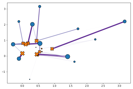
In the simple toy example below, we compute the optimal coupling matrix between two point clouds sampled randomly (2D vectors, compared with the squared Euclidean distance):
import jax
import jax.numpy as jnp

from ott.geometry import pointcloud
from ott.problems.linear import linear_problem
from ott.solvers.linear import sinkhorn

# sample two point clouds and their weights.
rngs = jax.random.split(jax.random.PRNGKey(0), 4)
n, m, d = 12, 14, 2
x = jax.random.normal(rngs[0], (n,d)) + 1
y = jax.random.uniform(rngs[1], (m,d))
a = jax.random.uniform(rngs[2], (n,))
b = jax.random.uniform(rngs[3], (m,))
a, b = a / jnp.sum(a), b / jnp.sum(b)
# Computes the couplings using the Sinkhorn algorithm.
geom = pointcloud.PointCloud(x, y)
prob = linear_problem.LinearProblem(geom, a, b)

solver = sinkhorn.Sinkhorn()
out = solver(prob)
The call to solver(prob) above works out the optimal transport solution. The out object contains a transport matrix
(here of size
If you have found this work useful, please consider citing this reference:
@article{cuturi2022optimal,
  title={Optimal Transport Tools (OTT): A JAX Toolbox for all things Wasserstein},
  author={Cuturi, Marco and Meng-Papaxanthos, Laetitia and Tian, Yingtao and Bunne, Charlotte and
          Davis, Geoff and Teboul, Olivier},
  journal={arXiv preprint arXiv:2201.12324},
  year={2022}
}
The moscot package for OT analysis of multi-omics data also uses OTT as a backbone.

