. 2017 Sep 12;20(11):2706-2718.
doi: 10.1016/j.celrep.2017.08.063.

A Mass Spectrometry-Based Approach for Mapping Protein Subcellular Localization Reveals the Spatial Proteome of Mouse Primary Neurons

Affiliations

A Mass Spectrometry-Based Approach for Mapping Protein Subcellular Localization Reveals the Spatial Proteome of Mouse Primary Neurons

Daniel N Itzhak et al. Cell Rep. .

Abstract

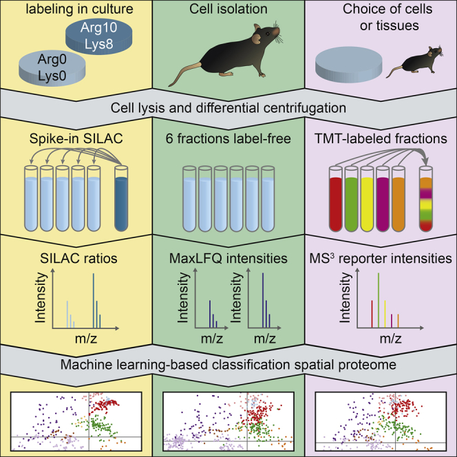
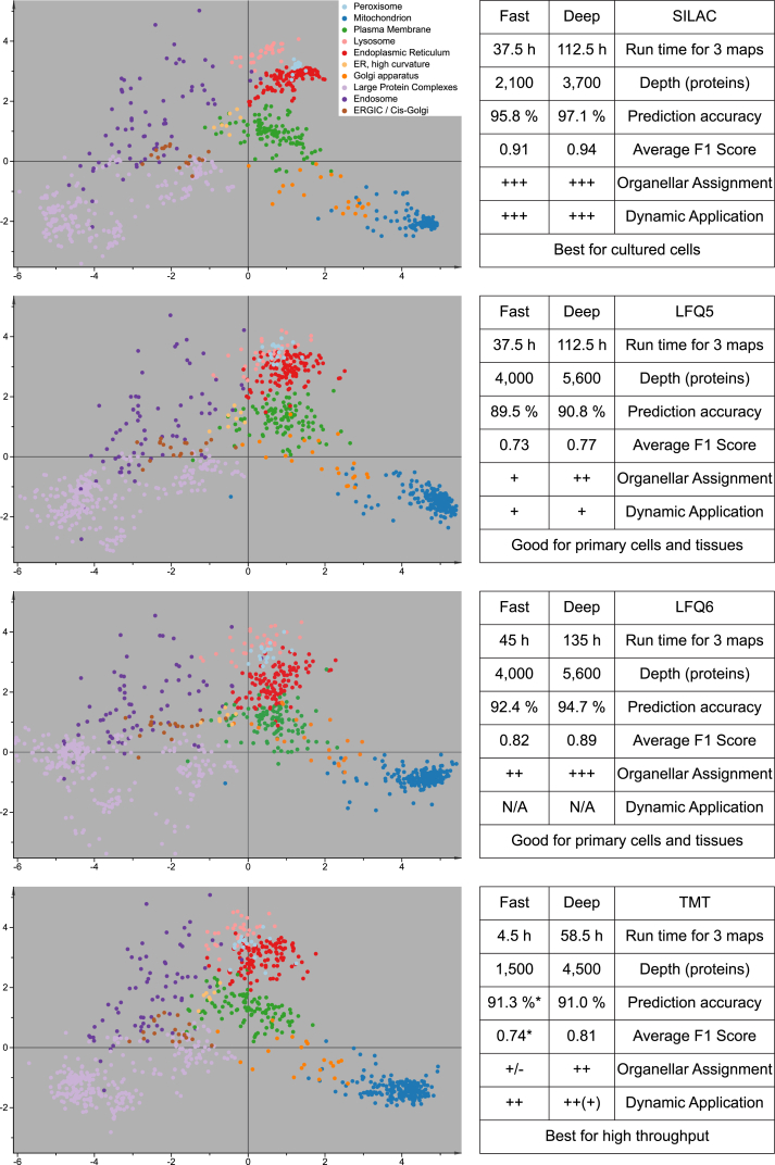
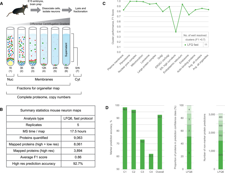
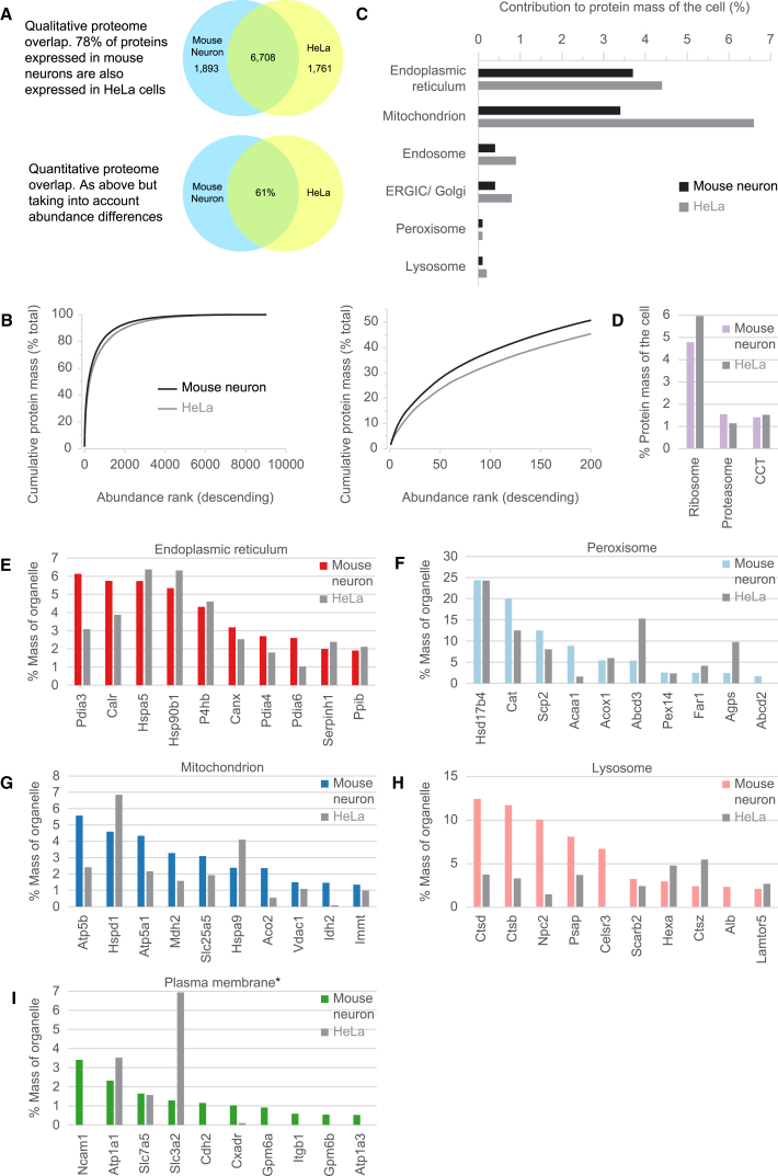
We previously developed a mass spectrometry-based method, dynamic organellar maps, for the determination of protein subcellular localization and identification of translocation events in comparative experiments. The use of metabolic labeling for quantification (stable isotope labeling by amino acids in cell culture [SILAC]) renders the method best suited to cells grown in culture. Here, we have adapted the workflow to both label-free quantification (LFQ) and chemical labeling/multiplexing strategies (tandem mass tagging [TMT]). Both methods are highly effective for the generation of organellar maps and capture of protein translocations. Furthermore, application of label-free organellar mapping to acutely isolated mouse primary neurons provided subcellular localization and copy-number information for over 8,000 proteins, allowing a detailed analysis of organellar organization. Our study extends the scope of dynamic organellar maps to any cell type or tissue and also to high-throughput screening.

Keywords: EGF signaling; LFQ; TMT; label-free quantification; neurons; organellar proteomics; primary cells; quantitative mass spectrometry; spatial proteomics; tandem mass tagging.


Figures

None
Graphical abstract
Figure 1
Figure 1
Workflow for Dynamic Organellar Maps Using Fractionation Profiling (A) In all workflows, whole-cell lysate was subjected to differential centrifugation to generate fractions enriched in different organelles. Note that the nuclear-enriched 1K fraction also contains a proportion of non-nuclear material. For the SILAC workflow, heavy-labeled post-nuclear supernatant was subjected to a single centrifugation step to generate a reference membrane fraction. Each of the fractions, excluding the 1K nuclear fraction, was combined 1:1 with the reference fraction and measured by MS. The SILAC ratios along the gradient generate profiles for each protein. In comparative experiments, the SILAC heavy reference fraction was from cells treated to match the fractionated material. (B) LFQ workflow. The same differential centrifugation as for SILAC light was used. Including the 1K nuclear-enriched fraction in the analysis increased separation of some organelles, as seen by comparing median organellar marker profiles (5 fractions, center, versus 6 fractions, right). Please note that inclusion of the 6th fraction also entails re-normalization of the profile to a sum of 1; this causes relative shifts in all fractions. (C) TMT workflow, which used identical fractions as the SILAC light workflow. Following protein digestion, peptides from each fraction were labeled with tandem mass tagging reagent and analyzed on an instrument capable of synchronous precursor selection-MS3 (SPS-MS3). TMT 10-plex permitted two maps to be measured in a single experiment. (D) Median profiles for organellar marker proteins are shown for three organelles with the different methods: SILAC (left), LFQ (center), and TMT (right). (E) As for (D), except profiles for the same organelle obtained with the different quantification strategies are shown.
Figure 2
Figure 2
Performance Analysis of Organellar Maps Generated with TMT, LFQ, and SILAC Quantification Strategies (A) To illustrate the relative precision of the different quantification methods applied in fractionation profiling, profile scatter within the 20S core proteasome (14 subunits, PSMA1–7, PSMB1–7, three independent measurements per protein) was analyzed (deep MS protocol). LFQ measurements are “noisier” than SILAC or TMT. Boxes indicate the interquartile range and whiskers 10th–90th percentile range. (B) Organellar classification performance of six independent LFQ-based maps. Accuracy is the proportion of correctly classified organellar markers during supervised learning. Performance was assessed for six-fraction profiles (LFQ6, green) and for the same maps with the sixth data point removed (LFQ5, yellow). (C) Combining several LFQ maps for organellar classification enhanced prediction accuracy. (Fast) maps shown in (B) were combined in the order of lowest to highest performance. Addition of each map improved performance. Maps 3, 4, and 6 were then chosen for further deep MS analysis and combined for classification. (D) Marker prediction accuracy obtained with a combination of three replicate maps by quantification strategy and MS protocol. TMT fast maps included predictions for only 10 of 12 clusters (see also Figure S1G). (E) Number of profiled proteins quantified in all three replicates. (F) MS measurement requirements (hours) for the generation of three replicate maps. (G–K) In-depth analysis of the predictions obtained with a combination of three replicate datasets, deep MS protocol (an equivalent analysis for predictions obtained with the fast MS protocol is shown in Figures S1B–S1E). (G) Detailed performance profiles of maps made with SILAC, LFQ5/6, and TMT. Prediction performance was evaluated for each organellar cluster. F1 scores were calculated as the harmonic mean of recall (true positives / [true positives + false negatives]) and precision (true positives / (true positives + false positives]). High F1 scores (> 0.7) denote clusters with a high predictive value. (H) Stratification of non-marker organellar predictions. Each assignment was made with a prediction confidence score. Four different SVM score cutoffs were defined, dividing the data into confidence classes. The prediction accuracy of marker proteins within each class served as a proxy for the prediction accuracy of non-marker proteins. Generally, the first two classes had high accuracies with all methods. (I and J) Proportion (I) and absolute number (J) of non-marker predictions in each confidence class. (K) Concordance analysis. The predictions of non-marker proteins, obtained with TMT, LFQ5, and LFQ6, were compared with the predictions obtained with SILAC. Concordance is the proportion of proteins with identical predictions. Restricting the comparison to proteins with a minimum confidence score in both compared maps reduces the overlapping dataset but increases concordance. In all cases, over 85% of the predictions show > 90% agreement. See also Figure S1 and Table S1.
Figure 3
Figure 3
Assessment of Dynamic Organellar Maps with Different Quantification Strategies Using the Deep MS Protocol (A) Three replicate SILAC experiments of cells left untreated or stimulated with EGF for 20 min were analyzed in a dynamic organellar maps experiment. The resulting difference profiles were subjected to statistical analysis to identify moving proteins (see Experimental Procedures for details). The movement and reproducibility scores for each protein are shown in an MR scatterplot; significantly moving proteins have high scores in both dimensions. The shaded area contains proteins where the estimated false discovery rate (FDR) for translocation is < 10% based on a mock control experiment. (B) Top: the proportion of EGFR in each fraction across the differential centrifugation gradient for three replicates in control cells (gray lines) or cells stimulated with EGF (black lines). Bottom: the difference in protein pelleting in the fractions in untreated compared with EGF-treated cells for three replicates. (C) Proteins in the shaded area of (A) were removed from the marker set, and all remaining proteins were subjected to organelle classification using SVM-based machine learning. The prediction scores for the plasma membrane and endosome are shown before and after treatment with EGF, correctly capturing the change in localization of the EGF receptor. (D–F) The same as (A)–(C), respectively, but for LFQ-based (deep) experiments. Note that the shaded area corresponds to a translocation FDR of < 20%. (G–I) Also the same as (A)–(C), respectively, but using data from the TMT-based (deep) experiments. Note that the shaded area is not FDR-controlled but uses cutoffs determined for the SILAC and LFQ experiments. See also Figures S2 and S3 and Table S2.
Figure 4
Figure 4
Visual Map Representation of 941 Marker Proteins Common to All Triplicate Deep Datasets (Left) and Key Metrics and Characteristics for Both Fast and Deep MS Protocols of the SILAC, LFQ5, LFQ6, and TMT Methods (Right) Plots for the SILAC, LFQ5, and TMT methods were generated from a single principal-component analysis, where each marker protein had three different entries, one for each of the methods, and each entry had fifteen data points corresponding to three replicates of five fractions. Because LFQ6 has an additional data point for each map, an independent PCA was used to generate this plot; it was then scaled for optimum comparison with the other methods. All maps show highly similar separation and orientation of marker protein clusters, with increased cluster density of SILAC relative to other methods, most evident with the peroxisomal cluster. Furthermore, note that each plot is a 2D representation of a 15-dimensional dataset (18-dimensional for LFQ6); many seemingly overlapping clusters are resolved in higher dimensions not illustrated here. TMT fast maps include predictions for only 10 subcellular localizations; all other maps include 12.
Figure 5
Figure 5
Application of Label-free Organellar Mapping to Mouse Neurons (A) Schematic workflow. Cortical neurons were acutely isolated from embryonic mice, lysed mechanically, and subjected to a series of differential centrifugation steps: 1, nuclear-enriched fraction; 2–6, membrane fractions; 7, cytosol. All fractions were analyzed by label-free quantitative mass spectrometry. Fractions 1–6 were used to generate organellar maps. Fractions 1, 2–6 combined, and 7 were used to quantify proteins’ nuclear, membrane-associated, and cytosolic pools. All fractions, 1–7 combined, were used to calculate protein copy numbers per cell. (B) Summary of neuron map performance (combined output from five independent replicates). (C) Detailed performance profiles of neuron maps. F1 scores were calculated as the harmonic mean of recall and precision, for each compartment, as in Figure 2G. (D) Stratification of non-marker organellar predictions as in Figure 2H. The prediction accuracy of marker proteins within each class served as a proxy for the prediction accuracy of non-marker proteins. The first two classes had very high accuracies. Proportion and absolute number of non-marker predictions in each confidence class are shown in the center and on the right, respectively. See also Figure S4 and Tables S3, S4, and S5.
Figure 6
Figure 6
Comparative Organellar Anatomy of Mouse Neurons and HeLa Cells (A) Full proteome overlap analysis. Top: qualitative overlap; the proportion of proteins detected in mouse neurons, with orthologs expressed in HeLa cells. Bottom: quantitative overlap (protein IDs and abundance considered). (B) Proteins detected in neurons (black) or HeLa cells (gray) were ordered by abundance. The cumulative contribution to total cell protein mass was plotted on the y axis. In both cases, the 100 most abundant proteins contribute over one-third of the total protein mass (right). (C) Relative contribution of individual organelles to total cell protein mass. Please note that the mouse neurons were acutely isolated; during this procedure, neurites, and, hence, parts of the plasma membrane, are lost (see Supplemental Experimental Procedures for details). This will lower the apparent plasma membrane contribution (which is not shown here for this reason) but is unlikely to substantially affect other organelles. (D) Abundant protein complexes make remarkably similar contributions to the total proteome in both cell types. CCT, a multi-subunit chaperonin, is also known as TRiC. (E–I) Compositional analysis of major organelles: (E) ER, (F) peroxisome, (G) mitochondrion, (H) lysosome, (I) plasma membrane. In each case, the ten most abundant proteins of the neuronal organelle were determined; the y axis shows their contributions to the total mass of the organelle. For comparison, the contributions of the same proteins to the corresponding HeLa organelles are shown (gray bars). Some organelles have extremely similar compositions (e.g., ER, peroxisome), others differ qualitatively (plasma membrane) or quantitatively (i.e., the same proteins but different distribution; e.g., lysosome). For the plasma membrane, only integral membrane proteins were considered. Although many synaptic marker proteins were detected in neuron lysates (Table S4), we did not observe a separate cluster corresponding to synapses.

Similar articles

Cited by

References

    1. Aebersold R., Mann M. Mass-spectrometric exploration of proteome structure and function. Nature. 2016;537:347–355. - PubMed
    1. Boisvert F.M., Ahmad Y., Gierlinski M., Charriere F., Lamont D., Scott M., Barton G., Lamond A.I. A quantitative spatial proteomics analysis of proteome turnover in human cells. Mol. Cell. Proteomics. 2012;11 M111.011429. - PMC - PubMed
    1. Christoforou A., Mulvey C.M., Breckels L.M., Geladaki A., Hurrell T., Hayward P.C., Naake T., Gatto L., Viner R., Martinez Arias A., Lilley K.S. A draft map of the mouse pluripotent stem cell spatial proteome. Nat. Commun. 2016;7:8992. - PMC - PubMed
    1. Cox J., Mann M. MaxQuant enables high peptide identification rates, individualized p.p.b.-range mass accuracies and proteome-wide protein quantification. Nat. Biotechnol. 2008;26:1367–1372. - PubMed
    1. Cox J., Hein M.Y., Luber C.A., Paron I., Nagaraj N., Mann M. Accurate proteome-wide label-free quantification by delayed normalization and maximal peptide ratio extraction, termed MaxLFQ. Mol. Cell. Proteomics. 2014;13:2513–2526. - PMC - PubMed

LinkOut - more resources