. 2017 Jan 1;66(1):e66-e82.
doi: 10.1093/sysbio/syw077.

Fundamentals and Recent Developments in Approximate Bayesian Computation

Affiliations

Fundamentals and Recent Developments in Approximate Bayesian Computation

Jarno Lintusaari et al. Syst Biol. .

Abstract

Bayesian inference plays an important role in phylogenetics, evolutionary biology, and in many other branches of science. It provides a principled framework for dealing with uncertainty and quantifying how it changes in the light of new evidence. For many complex models and inference problems, however, only approximate quantitative answers are obtainable. Approximate Bayesian computation (ABC) refers to a family of algorithms for approximate inference that makes a minimal set of assumptions by only requiring that sampling from a model is possible. We explain here the fundamentals of ABC, review the classical algorithms, and highlight recent developments. [ABC; approximate Bayesian computation; Bayesian inference; likelihood-free inference; phylogenetics; simulator-based models; stochastic simulation models; tree-based models.]


Figures

Figure 1.
Figure 1.
Illustration of the stochastic simulator formula image run multiple times with a fixed value of formula image. The black dot formula image is the observed data and the arrows point to different simulated data sets. Two outcomes, marked in green, are less than formula image away from formula image. The proportion of such outcomes provides an approximation of the likelihood of formula image for the observed data formula image.
Figure 2.
Figure 2.
An example of a transmission process simulated under a parameter configuration formula image without subsampling of the simulated infectious population. Arrows indicate the sequence of random events taking place in the simulation and different colors represent different haplotypes of the pathogen. The simulation starts with one infectious host who transmits the pathogen to another host. After one more transmission event, the pathogen undergoes a mutation within one of the three hosts infected so far (event three). As the sixth event in the simulation, one of the haplotypes is removed from the population due to the recovery/death of the corresponding host. The simulation stops when the infectious population size exceeds formula image and the simulator outputs the generated formula image. The nodes not connected by arrows show all the other possible configurations of the infectious population, but which were not visited in this example run of the simulator. The bottom row lists the possible outputs of the simulator (cluster size vectors) under their corresponding population configuration.
Figure 3.
Figure 3.
The transmission process in Figure 2 can also be described with transmission trees (Stadler 2011) paired with mutations. The trees are characterized by their structure, the length of their edges, and the mutations on the edges (marked with small circles that change the color of the edge, where colors represent the different haplotypes of the pathogen). The figure shows three examples of different trees that yield the same observed data at the observation time formula image. Calculating the likelihood of a parameter value requires summing over all possible trees yielding the observed data, which is computationally impossible when the sample size is large.
Figure 4.
Figure 4.
Exact inference for a simulator-based model of tuberculosis transmission. A very simple setting was chosen where the exact posterior can be numerically computed (black line), and where Algorithm 1 is applicable (blue bars).
Figure 5.
Figure 5.
Inference results for the transmission rate formula image of tuberculosis. The plots show the posterior distributions obtained with Algorithm 2 and 20 million simulated data sets (proposals). a) Cluster frequency as a summary statistic. b) Genetic diversity as a summary statistic.
Figure 6.
Figure 6.
Comparison of the efficiency of Algorithms 1 and 2. Smaller KL divergence means more accurate inference of the posterior distribution. Note that the stopping criterion of the algorithm has here been changed to be the total number of runs of the simulator instead of the number of accepted samples. a) Results after 100,000 simulations. b) Accuracy versus computational cost.
Figure 7.
Figure 7.
Comparison of the trade-off between Monte Carlo error and bias. Algorithm 1 is equivalent here to Algorithm 2 with formula image. Smaller KL divergences mean more accurate inference of the posterior distribution. a) Results after 100,000 simulations. b) Accuracy versus computational cost.
Figure 8.
Figure 8.
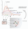
Illustration of sequential Monte Carlo ABC using the tuberculosis example. The first proposal distribution is the prior and the threshold value used is formula image. The proposal distribution in iteration formula image is based on the sample of size formula image from the previous iteration. The threshold value formula image is decreased at every iteration as the proposal distributions become similar to the true posterior. The figure shows parameters drawn from the proposal distribution of the third iteration (formula image). The red proposal is rejected because the corresponding simulation outcome is too far from the observed data formula image. At iteration formula image, however, it would have been accepted. After iteration formula image, the accepted parameter values follow the approximate posterior formula image. As long as the threshold values formula image decrease, the approximation becomes more accurate at each iteration.
Figure 9.
Figure 9.
Illustration of the linear regression adjustment (Beaumont et al. 2002). First, the regression model formula image is learned and then, based on formula image, the simulations are adjusted as if they were sampled from formula image with formula image. Note that the residuals formula image are preserved. The change in the posterior densities after the adjustment is shown on the right. Here, the black (original) and green (adjusted) curves are the same as in Figure 10(b).
Figure 10.
Figure 10.
Linear regression adjustment (Beaumont et al. 2002). applied to the example model of the spread of tuberculosis (compare to Fig. 5). The target distribution of the adjustment is the posterior formula image with the threshold decreased to formula image. Note that when using summary statistic formula image the target distribution is substantially different from the true posterior (reference) because of the bias incurred by formula image. a) formula image with formula image. b) formula image with formula image.
Figure 11.
Figure 11.
The basic idea of BOLFI is to model the distance, and to prioritize regions of the parameter space where the distance tends to be small. The solid curves show the modeled average behavior of the distance formula image, and the dashed curves its variability for the tuberculosis example. a) After initialization (30 data points). b) After active data acquisition (200 data points).
Figure 12.
Figure 12.
In BOLFI, the estimated model of formula image is used to approximate formula image by computing the probability that the distance is below a threshold formula image. This kind of likelihood approximation leads to a model-based approximation of formula image. The KL-divergence between the reference solution and the BOLFI solution with 30 data points is 0.09, and for 200 data points it is 0.01. Comparison with Figure 6 shows that BOLFI increases the computational efficiency of ABC by several orders of magnitude. a) Approximate likelihood function. b) Model-based posteriors.

Similar articles

Cited by

References

    1. Aeschbacher S., Beaumont M., Futschik A. 2012. A novel approach for choosing summary statistics in approximate Bayesian computation. Genetics 192:1027–1047. - PMC - PubMed
    1. Anderson R.M., May R.M. 1992. Infectious diseases of humans: dynamics and control. Oxford University Press.
    1. Barber S., Voss J., Webster M. 2015.. The rate of convergence for approximate Bayesian computation. Electron. J. Stat. 80–105.
    1. Baudet C., Donati B., Sinaimeri B., Crescenzi P., Gautier C., Matias C., Sagot M.-F. 2015.. Cophylogeny reconstruction via an approximate Bayesian computation. Syst. Biol. 64:416–431. - PMC - PubMed
    1. Beaumont M.A. 2010.. Approximate Bayesian computation in evolution and ecology. Annu. Rev. Ecol. Evol. Syst. 41:379–406.

Publication types